

https://www.nature.com/articles/s41528-023-00289-6
Project Profile
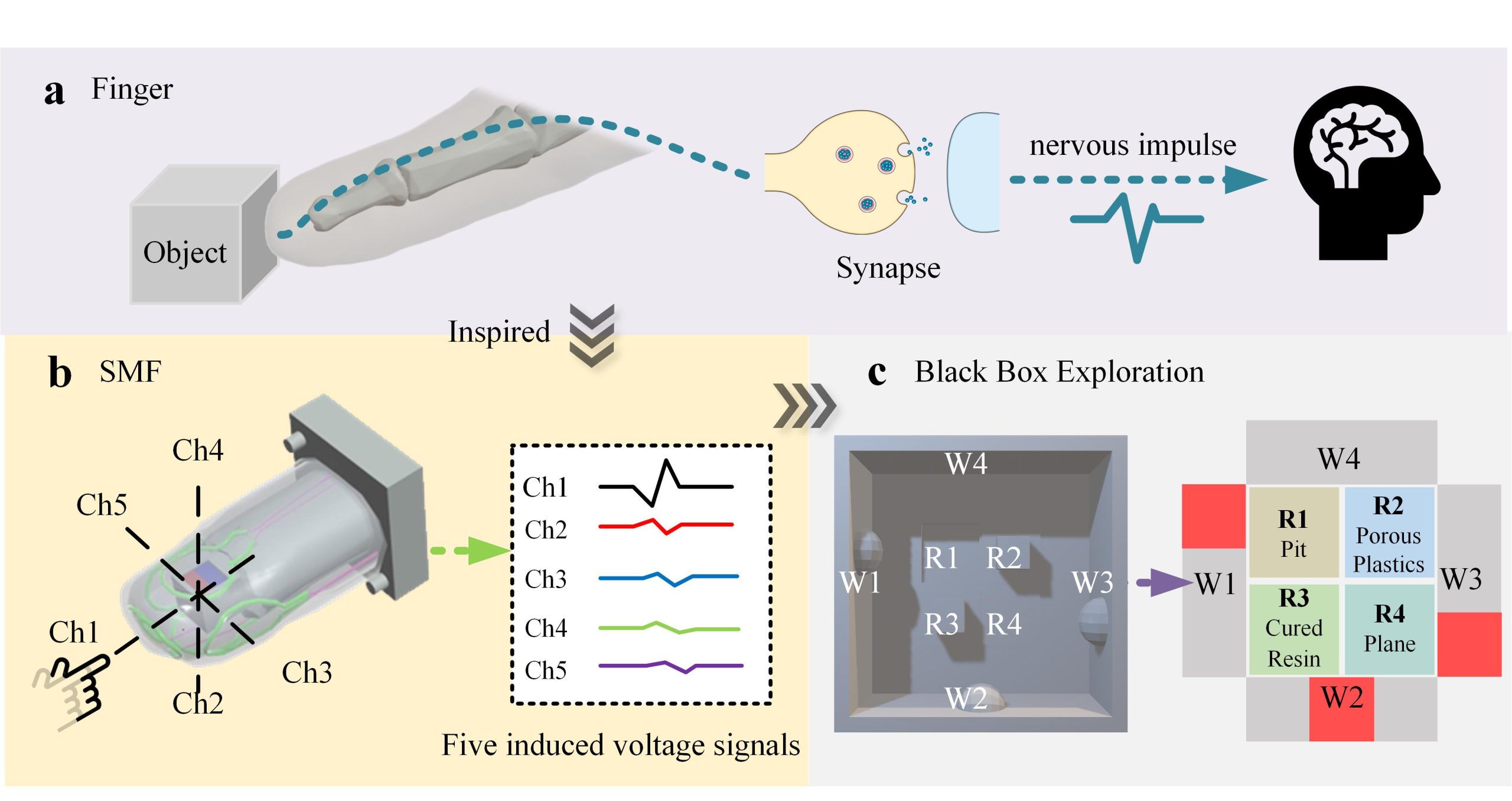
This project was part of my personal master’s project and I was responsible for the entire program which demonstrated a Soft Magnetoelectric Finger (SMF) which can achieve self-generated-signal and multidirectional tactile sensing. As shown in Figure 1, the structure of the SMF is inspired by the skin-bone structure of the human finger and is composed of 2 parts: a ‘finger’ covered with a skin-like flexible sheath containing five liquid metal coils and a ‘phalangeal bone’ containing a magnet. According to electromagnetic induction, different electrical signals will be generated on the five coils due to the changes in magnetic flux through those coils when suffer varied forces, Abaqus and Maxwell were chosen to simulate this process. Besides, we also dug into the potential of the SMF in multidirectional sensing and object recognition by the detailed analysis of the signals. Here, I would like to briefly introduce this project in three aspects: Simulation, Multidirectional sensing, and Object recognition. Some descriptions are excerpted from the manuscript.

Simulation
Numerical analysis via Abaqus and Maxwell was performed to explain the sensing mechanism. The model including ‘finger ‘ and ‘phalangeal bone’ were created by 3d max. The Abaqus 6.14-4 was used to calculate the shape deformations of the SMF when suffering a vertical force. Subsequently, the original and deformed models were imported to the Ansys Maxwell finite element analysis software, which was used to conduct 3D modeling of a NdFeB magnetic cube integrated with LM rings, and calculate the distribution of magnetic intensity before and after deformation.
Shape Deformation of the SMF
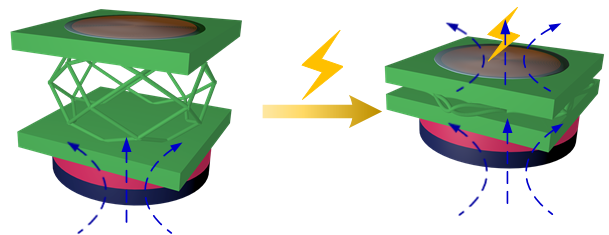
“The software Abaqus/CAE was used to conduct the shape deformations of the SMF when the Ch1 was pressed. The elastic film with five microchannels was positioned between the rigid bone and a rigid plate (hiden), and the hard contact in normal behavior was set. The rigid plate was used for vertical compression while the boundary conditions with encastre were applied for the bone. The parameters for the simulation were used according to similar rubber material to: density of 1.18 g/cm3, Young’s modulus of 1.5 MPa, and Poisson’s ratio of 0.25.”* Video 1 shows the process of SMF being pressed.
Distribution of Magnetic Intensity

“The ANSYS MAXWELL finite element analysis software was used to conduct the distribution of magnetic intensity of a magnet (a cube with 5 mm in side length) integrated with liquid metal coils. In this study, the magnetic coercivity was set as -954929.6 A·m−1, as well as residual flux density of ~1.2 T. In the simulation modeling, several assumed conditions should be taken into consideration, as follows:
- The five liquid metals coils involved in this experiment were simplified as the equivalent coils based on the microchannels on the film surface before and after deformation.
- The liquid metals coils are in an infinite vacuum.”
As a result, the simulated distribution of magnetic intensity for the liquid metal-based coils before/after compression was shown in Figure 2.
”The total magnetic flux of each coil before/after compression can be calculated according to the following equation below:
E(V)=-∆Φ/∆t=-(Φ_((after) )-Φ_((before) ))/∆twhere E(V) is the output voltage, ΔΦ is the total magnetic flux change, and Δt is the response time of the sheath.
The calculated induced voltages in each coil matched the experimental results, and the difference between the experimental result and the theoretical one is mainly caused by the position differences of LM coils between calculated and actual conditions.“
Multidirectional sensing

“The multidirectional tactile sensing capability of the SMF comes from the spatial arrays of five LM coils surrouding the magnet, besides normal pressures, the spatical arrangement of the five LM coils enables the SMF to distinguish shear forces towards diverse directions.”
Taking Ch4 as an example (as shown in Figure 3 left), in addition to the forces on the center of the Ch4 side, the SMF can also distinguish shear forces from the Ch4 side to the Ch3 side (in short 4→3, see Figure 3 right), 4→1, and 4→5. This is because these different forces cause the spatial array of LM coils to generate different sets of induced voltage signals, and by analyzing these different sets of signals in detail, the SMF is able to discriminate between forces in different directions far beyond the density of sensitive units.
Object recognition

“The SMF was used to recognize different objects with diverse Young’s moduli. Six common objects were selected as test subjects, including sponge cube, porous plastics, paperboard, foamed plastics, Ecoflex rubber, and cured resin, as shown in Figure 4a. … The SMF was integrated into the compression platform to touch these objects at a speed of 10 mm/s and a displacement of 3.5 mm for 360 times (pulse-like mechanical stimulation). … Since the six groups of objects have different Young’s moduli, varied degrees of shape deformation occurred when they were touched by the SMF at the same deformation, resulting in different induced voltage signals of Ch1. In order to achieve accurate identification of these objects, machine learning algorithms were introduced accordingly.
The flowchart of machine learning is shown in Figure 4b. Since the compressions occurred coherently during the experiment, the raw data of each acquired object was divided into 120 strips, that is, about 3 times of compressions in a group to ensure the integrity of the information and labeled them according to categories. For each object, 80% (96 groups) of the data was selected as the training set, and the remaining 20% (24 groups) was known as the test set. In the end, the training set had a total of 576 pieces of data and the test set had a total of 144 pieces of data.
For this multiclass problem, tests were conducted on five different machine learning algorithms using the same dataset. Among them, the LightGBM classifier achieved the highest accuracy rate of 97.46% in classifying six different objects. The test results of the confusion matrix for the LightGBM classifier are shown in Figure 4d.
To facilitate a more intuitive representation of the signal disparities among the six materials, the T-SNE (t-Distributed Stochastic Neighbor Embedding) algorithm was applied for data visualization. T-SNE is a robust nonlinear technique widely employed for reducing dimensionality and visualizing high-dimensional datasets. The resulting plot in Figure 4c demonstrates notable clustering patterns among the six materials, indicating promising prospects for utilizing machine learning in material classification endeavors.”
Brief Conclusion
This page provides a brief overview of the SMF in three areas: Simultaion, Multidirectional sensing and object recognition. In Addition to this, there is a lot of other related work has been done. Related papers are currently under review.